Ensemble learning - stacking models with scikit-learn
What is ensembling
Ensembling is a ML technique in which we use multiple learning algorithms to get better performance than could be obtained from any of the algorithms alone.
There are many ways in which you could perform ensembling:
- voting classifiers,
- bagging,
- boosting,
- and stacking.
I will focus on the last method - stacking, which is based on a simple idea: to train a model to perform an aggregation of other models predictions. Moreover I will train it using out-of-fold predictions which I think has many advantages over alternative approaches.
This post is not so much about exploring the data or using state of the art algorithms. I will use simple models on barely preprocessed data without any tuning. There are many improvements that could be done to the presented pipeline in this regard, but that’s not the main focus of the post. You can skip right to the ensembling part or read also about:
- inspecting the data and drawing simple visualizations
- constructing pipelines for data preprocessing
Let’s start.
Data loading and visualization
First we need to import numpy and pandas - libraries for numerical data processing and sklearn for a rich source of machine learning models. I will also set the numpy seed (basically a number that determines what pseudo-number variables will be generated by numpy) for deterministic runs. Repeatability is a very important thing when there is so many moving parts.
import pandas as pd
import numpy as np
import sklearn

np.random.seed(42)
data_dir = "datasets/house_prices"
First, let’s load the data into pandas DataFrame. The dataset comes from the Kaggle learning competition: https://www.kaggle.com/c/house-prices-advanced-regression-techniques, which aim is to make the best predictor for house selling prices.
housing = pd.read_csv(data_dir + '/train.csv')
Now let’s just briefly take a look at the data.
housing.info()
<class 'pandas.core.frame.DataFrame'>
RangeIndex: 1460 entries, 0 to 1459
Data columns (total 81 columns):
Id               1460 non-null int64
MSSubClass       1460 non-null int64
MSZoning         1460 non-null object
LotFrontage      1201 non-null float64
LotArea          1460 non-null int64
Street           1460 non-null object
Alley            91 non-null object
LotShape         1460 non-null object
LandContour      1460 non-null object
Utilities        1460 non-null object
...
3SsnPorch        1460 non-null int64
ScreenPorch      1460 non-null int64
PoolArea         1460 non-null int64
PoolQC           7 non-null object
Fence            281 non-null object
MiscFeature      54 non-null object
MiscVal          1460 non-null int64
MoSold           1460 non-null int64
YrSold           1460 non-null int64
SaleType         1460 non-null object
SaleCondition    1460 non-null object
SalePrice        1460 non-null int64
dtypes: float64(3), int64(35), object(43)
memory usage: 924.0+ KB
As you can see there are some columns with many missing values. One of the options in this case (certainly the simplest) is to entirely drop them, and that’s what we’re going to do.
housing.drop(['MiscFeature', 'Fence', 'PoolQC',
              'FireplaceQu', 'Alley', 'Id'], inplace=True, axis=1)
Now let’s split the data into 3 subsets:
- training set,
- validation set for tuning hyperparameters,
- test set for final testing
We set the random_state to 42 so that the subsets contain the same data every time we run the code.
from sklearn.model_selection import train_test_split

train_val_set, test_set = train_test_split(housing, test_size=0.2, random_state=42)
train_set, val_set = train_test_split(train_val_set, test_size=0.2, random_state=42)
Now it’s time to take a closer look and get some insights from the data. Let’s use describe method of DataFrame to compute some basic statistics.
housing[['YearBuilt', 'LotArea', 'SalePrice', 'GrLivArea']].describe()
.dataframe td, .dataframe th {
border-left: 0px; border-right: 0px; }
.dataframe tbody tr th {
    vertical-align: top;
}

.dataframe thead th {
    text-align: left;
}
To see the data distribution let’s call hist method of DataFrame:
%matplotlib inline
import matplotlib.pyplot as plt
train_set[['YearBuilt', 'LotArea', 'OverallQual', 'GrLivArea',
           'BedroomAbvGr', 'SalePrice']].hist(bins=50, figsize=(20,15))
plt.show()
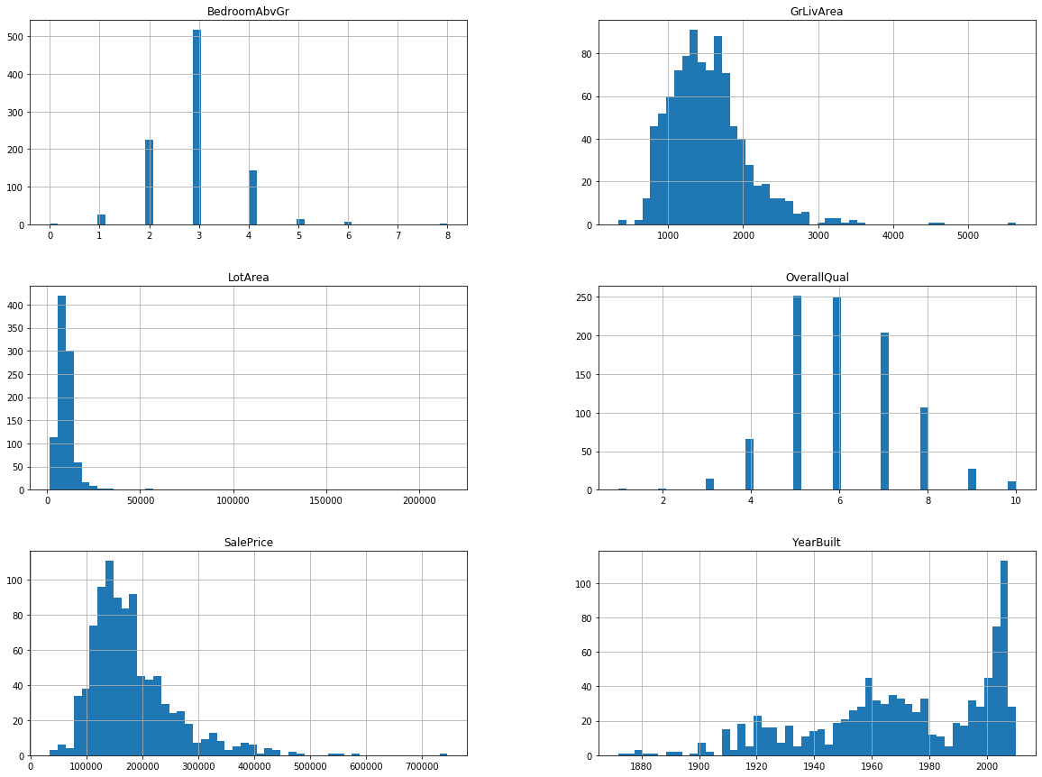
You can see that the data is not exactly normally distributed, in some cases the tails are quite long e.g for SalePrice. We could try to transform them e.g take a logarithm or even remove the outliers, but in this case let’s just keep them as they are.
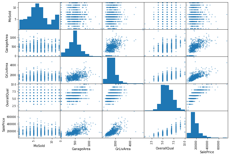
Scatter plots and correlations are a good way to pinpoint important variables. Let’s see which of the columns seem to be correlated to the target variable - SalePrice
corr_matrix = train_set.corr()
corr_matrix["SalePrice"].sort_values(ascending=False)
SalePrice        1.000000
OverallQual      0.777892
GrLivArea        0.674807
GarageCars       0.637454
GarageArea       0.616631
TotalBsmtSF      0.593411
1stFlrSF         0.588018
FullBath         0.550514
YearBuilt        0.515217
TotRmsAbvGrd     0.508304
YearRemodAdd     0.492897
GarageYrBlt      0.479604
Fireplaces       0.464652
MasVnrArea       0.440977
BsmtFinSF1       0.351121
LotFrontage      0.313306
WoodDeckSF       0.307913
2ndFlrSF         0.284592
OpenPorchSF      0.281425
HalfBath         0.266244
LotArea          0.239065
BsmtUnfSF        0.229066
BsmtFullBath     0.228611
BedroomAbvGr     0.157942
ScreenPorch      0.139919
PoolArea         0.131198
3SsnPorch        0.090449
MoSold           0.017851
BsmtFinSF2       0.010182
LowQualFinSF     0.009869
YrSold           0.003952
MiscVal         -0.020882
BsmtHalfBath    -0.045244
MSSubClass      -0.088854
OverallCond     -0.095197
EnclosedPorch   -0.133094
KitchenAbvGr    -0.137487
Name: SalePrice, dtype: float64
Variables OverallQual or GrLivArea seem to be correlated with the results and when you think about it, it makes sense that quality and area will positively affect the price. There are also some variables that seem to be weakly correlated like MoSold. They are candidates for variables to drop from dataset. Also the variables strongly correlated with some other variables (not target variable) might be sometimes removed benefiting the model performance. For now we’ll just let them be.
We can also plot some of the variables together to get some better insights:
from pandas.plotting import scatter_matrix

attributes = ['MoSold', 'GarageArea', 'GrLivArea', 'OverallQual', 'SalePrice']
_ = scatter_matrix(train_set[attributes], figsize=(12, 8))
Preprocessing the data
Now let’s clean up the data. We need to do a few things before we can move on:
- we have to split data sets into predictor and target columns,
- the numerical variables seem to be in different scales, we need to normalize them, as many of the algorithms work much worse on such data,
- some of the variables have missing values, we need to either fill them or drop the rows containing the missing data,
- factors (categorical values) need to be transformed to numerical values
We’ll put all of these steps into scikit-learn pipeline, so we can keep our sanity and ensure all the parts of the datasets are processed the same way.
First let’s separate target variables and split numerical variables from factor variables:
from sklearn.preprocessing import StandardScaler
from sklearn.impute import SimpleImputer
from sklearn.pipeline import Pipeline
from sklearn.preprocessing import OneHotEncoder
def to_Xy(data_set):
    X = data_set.drop(['SalePrice'], axis=1)
    y = data_set['SalePrice'].copy()
    return X, y

train_X, train_y = to_Xy(train_set)
numeric_cols_selector = (train_X.dtypes == np.float64) | \
    (train_X.dtypes == np.int64)

numeric_cols = train_X.columns[numeric_cols_selector]

categorical_cols = train_X.columns[~numeric_cols_selector]
num_pipeline = Pipeline([
    ('imputer', SimpleImputer(strategy="median")),
    ('std_scaler', StandardScaler()),
])
SimpleImputer will fill the NaNs (missing values) with median and StandarScaler will change each value in train_X to z = (x - u) / s where u is the mean and s is the standard deviation of the training samples. Moreover both of them will store the parameters which they used so that later we can call scaler.transform on the validation / test set and apply the same transformations to them.
cat_pipeline = Pipeline([
    ('imputer', SimpleImputer(strategy="constant", fill_value='N/A')),
    ('encoder', OneHotEncoder(sparse=False, handle_unknown='ignore'))
])
For the categorical attributes we will use SimpleImputer again just to fill them with "N/A" string, and next all the factors will be transformed into the one-hot numerical encoding. It basically means that a factor column with 3 possible values will be transformed into a 3 columns of 0s and 1s e.g:
['cat', 'dog', 'dog', 'mouse'] => [[1, 0, 0], [0, 1, 0], [0, 1, 0], [0, 0, 1]]
Let’s apply the full pipeline now:
from sklearn.compose import ColumnTransformer

full_pipeline = ColumnTransformer([
        ("num", num_pipeline, numeric_cols),
        ("cat", cat_pipeline, categorical_cols),
    ])

p_train_X = full_pipeline.fit_transform(train_X)
To assess our models we’ll use the metric from the Kaggle competition which is root of mean squared error of logarithm (note that lower is better in this case):

from sklearn.metrics import mean_squared_error

def score_root_rmse(y_hat, y):
    return np.sqrt(mean_squared_error(np.log(y_hat), np.log(y)))

def scorer_neg_root_rmse(estimator, X, y):
    y_hat = estimator.predict(X)
    return -score_root_rmse(y_hat, y)
def print_res(res):
    print('Mean: {} Std: {} Scores: {}'.format(np.mean(res), np.std(res), res))
Now it’s time to use the first model. We will train regression model - ElasticNet. We will use cross_val_score function, which will perform cross-validation, to assess how good the model is.
Cross-validation works as follows: we split the dataset into N non-overlapping parts. In this case we will split the data into 5 parts. We will train 5 models, each on different 4/5 of the data and then we will make a prediction on the rest 1/5 of the data. Next the 5 partial predictions will be scored, and their scores averaged to give us a good estimate of how the final model will perform.
Here’s the simple visualization:
.dataframe tbody tr th {
    vertical-align: top;
}

.dataframe td, .dataframe th {
border-left: 0px; border-right: 0px; }
.dataframe thead th {
    text-align: left;
}
from sklearn.model_selection import KFold
from sklearn.linear_model import ElasticNet
from sklearn.model_selection import cross_val_score

enet = ElasticNet()

scores = cross_val_score(enet, p_train_X, train_y,
                         cv=KFold(n_splits=5, shuffle=True, random_state=42),
                         scoring=scorer_neg_root_rmse)
print_res(-scores)
Mean: 0.1485260220222559 Std: 0.01872265830761075 Scores: [0.17393527 0.16631658 0.1358159 0.12422032 0.14234204]
Now let’s try another model - DecisionTreeRegressor:
from sklearn.tree import DecisionTreeRegressor
d_tree = DecisionTreeRegressor(max_depth=5, random_state=42)
scores = cross_val_score(d_tree, p_train_X, train_y,
                         cv=KFold(n_splits=5, shuffle=True, random_state=42),
                         scoring=scorer_neg_root_rmse)
print_res(-scores)
Mean: 0.21493418568389946 Std: 0.0292174530898645 Scores: [0.25177622 0.19475781 0.2101796 0.17426314 0.24369416]
As you can see ElasticNet performs better than DescisionTreeRegressor. Both of the models have many hyperparameters that can be tuned using e.g. RandomizedSearchCV in order to find the best ones. We’ll settle for the default ones for now.
Now let’s score the models on validation set:
val_X = val_set.drop(['SalePrice'], axis=1)
val_y = val_set['SalePrice'].copy()
p_val_X = full_pipeline.transform(val_X)
enet = ElasticNet()
enet.fit(p_train_X, train_y)

enet_t_pred = enet.predict(p_val_X)
score_root_rmse(enet_t_pred, val_y)
0.14861355778098653
d_tree = DecisionTreeRegressor(max_depth=5, random_state=0)
d_tree.fit(p_train_X, train_y)

d_tree_t_pred = d_tree.predict(p_val_X)
score_root_rmse(d_tree_t_pred, val_y)
0.2084596276758006
Ensembling
Now let’s get to the main dish and try building an ensemble model using stacking. Basically it means combining the predictions of a set of models using some other model (called a blender or meta learner). We can repeat this as much as we want, creating deeper and deeper ensembles containing many layers of models.
Very important aspect of building an ensemble like this is careful feeding the data to each model so that we don’t leak the target variable when training on the previous results, which may lead to overly optimistic estimates of model performance and overfitting.
Out-of-fold predictions can be used to construct the training set for the meta learner with the same number of samples as the original training set.
In this case we will train the model using ElasticNet and DecisionTreeRegressor out-of-fold predictions.
What do I exactly mean by that? If you look at the table with cross-validation splits and then imagine taking the 5 partial predictions, but this time instead of using them to score the models, just concatenate them and use them as a training input for the blender model.
.dataframe td, .dataframe th {
border-left: 0px; border-right: 0px; }
.dataframe tbody tr th {
    vertical-align: top;
}

.dataframe thead th {
    text-align: left;
}
k_fold = KFold(n_splits=5, shuffle=True, random_state=42)
fold5 = list(k_fold.split(train_X))
Stacking will usually get us the best results if the underlying models differ at least a bit from each other (more is better). We can check that difference computing Pearson’s correlation between their predictions.
from scipy.stats import pearsonr
pearsonr(enet_t_pred, d_tree_t_pred)
(0.8595179258740466, 1.4397523477492039e-69)
As you can see the models are not exactly aligned (correlation less than 1) so it’s worth a shot.
l2_cols = ['tree', 'elastic_net']

l2_train_X = pd.DataFrame(0, index=np.arange(len(train_X)), columns=l2_cols)

fold_scores = {}

for train_idx, test_idx in fold5:
    X_fold_train = np.take(p_train_X, train_idx, axis=0)
    X_fold_test = np.take(p_train_X, test_idx, axis=0)
    y_fold_train = np.take(train_y, train_idx, axis=0)
    y_fold_test = np.take(train_y, test_idx, axis=0)
    for i, col in enumerate(l2_cols):
        if col == 'tree':
            fold_model = DecisionTreeRegressor(max_depth=4, random_state=0)
        else:
            fold_model = ElasticNet(max_iter=1000)
        _ = fold_model.fit(X_fold_train, y_fold_train)
        fold_pred = fold_model.predict(X_fold_test)
        l2_train_X.iloc[test_idx, i] = fold_pred
        fold_score = score_root_rmse(fold_pred, y_fold_test)
        fold_scores.setdefault(col, []).append(fold_score)
Now the l2_train_X variable contains the two columns - out-of-fold predictions from ElasticNet and DecisionTreeRegressor which will be used for training the combining model. We’ll use the ElasticNet and then score it on the validation set:
e_net_l2 = ElasticNet()
e_net_l2.fit(l2_train_X, train_y)

data_df = {'tree': d_tree_t_pred, 'elastic_net': enet_t_pred }
l2_val_X = pd.DataFrame(data=data_df, columns=l2_cols)

-scorer_neg_root_rmse(e_net_l2, l2_val_X, val_y)
0.1441181739070541
As you can see the model scored better than any of the underlying models on validation set. How do we now though that simply averaging the predictions wouldn’t work better? It’s good to have most basic baselines to see whether our “sophisticated” approach is worth all the work. Let’s see:
score_root_rmse(l2_val_X.mean(axis=1), val_y)
0.1585846156546493
Our approach is better! Let’s now see if we get good results on the holdout test set, which is a final test of our model performance.
test_X = test_set.drop(['SalePrice'], axis=1)
test_y = test_set['SalePrice'].copy()
p_test_X = full_pipeline.transform(test_X)
print('elastic_net', -scorer_neg_root_rmse(enet, p_test_X, test_y))
print('tree', -scorer_neg_root_rmse(d_tree, p_test_X, test_y))
elastic_net 0.1593466841918364
tree 0.2081436275107539
df_data = {
    'tree': d_tree.predict(p_test_X),
    'elastic_net': enet.predict(p_test_X)
}
l2_test_X = pd.DataFrame(data=df_data, columns=l2_cols)
-scorer_neg_root_rmse(e_net_l2, l2_test_X, test_y)
0.15004263401083465
It’s a bit worse than on validation set but still outperforms the underlying models without any tuning.
Examples of what not to do
There are things you might be tempted to do when approaching the ensembling problem, but trust me they won’t work as well. Two examples are:
- to train ensembling model on validation set predictions,
- to train ensembling model on the training set predictions
Problem with the first one is that we’re training ensemble on much less data than in the out-of-fold approach, so unless we have a lot of data and we can spare a big chunk of it for training the blender model, we’re better of doing it the shown way.
The problem with the second one is that we’re overfitting the training set, which is almost never a thing you really want.
Let’s see how these approaches will perform on the data.
Let’s check the first alternative approach:
e_net_l2_alt = ElasticNet()

scores = cross_val_score(e_net_l2_alt, l2_val_X, val_y,
                         cv=KFold(n_splits=5, shuffle=True, random_state=42),
                         scoring=scorer_neg_root_rmse)
print_res(-scores)
e_net_l2_alt = ElasticNet()
e_net_l2_alt.fit(l2_val_X, val_y)
-scorer_neg_root_rmse(e_net_l2_alt, l2_test_X, test_y)
Mean: 0.1521426949031468 Std: 0.02023885620633598 Scores: [0.15963401 0.13946745 0.13891518 0.18861394 0.1340829 ]
0.15636764734694825
… and now the second one:
df_data = {
    'tree': d_tree.predict(p_train_X),
    'elastic_net': enet.predict(p_train_X)
}

l2_train_X_x2 = pd.DataFrame(data=df_data,columns=l2_cols)

e_net_l2_alt_d = ElasticNet()
e_net_l2_alt_d.fit(l2_train_X_x2, train_y)
print(-scorer_neg_root_rmse(e_net_l2_alt_d, l2_val_X, val_y))
-scorer_neg_root_rmse(e_net_l2_alt_d, l2_test_X, test_y)
0.15961119338739369
0.16021217713329372
As you can see both of the alternative approaches scored worse than the recommended one, and I think it will be the case in most of the models you build.
That’s it. I hope you learned one or two things about ensembling from this post. Thanks for reading.
TL;DR Use out-of-fold predictions to train the model ensembles.